A No-BS Look at Quantitative Trading Infrastructure

Everyone wants to be a quant… until they’re skipping meals to pay their cloud bill.

At The Quant’s Playbook, we typically focus on building brand-new quantitative trading strategies from scratch, putting them through rigorous tests, and deploying them in real markets to make money. However, that’s only one part of the equation when it comes to building a real quantitative trading outfit.

This post won’t be our typical strategy or live market exploration — this one’s more about the overlooked backend foolery that keeps the machine churning.

We’re going to take a much-needed look behind the curtain at how managing data works in a real, mid-frequency quant setup.

We’re not HFT, so there won’t be things like microwave signals or ultra high-speed tech, but there’s still plenty of interesting ground to cover.

So, without further ado, let’s get into it.

“90% of the game is wrangling data, only 10% is actually trading.”

Medium-frequency trading (MFT) is loosely defined as having a holding period ranging from a few minutes to a few months. Some might define it differently, but for our purposes, that’s the timeframe we’re referring to when we talk about MFT.

If you’re trading on this timeframe, your data needs start off fairly simple: your basic, garden-variety OHLCV data, like this:

You typically just need the raw historical prices to test whatever idea you have, and then you go on about your day.

However, over time, you start to realize that the price data of a single stock over a single time period is essentially meaningless on its own.

Substantially more information can be found on a cross-sectional basis — not just how this stock performed, but how it performed relative to a bunch of others and across different time periods.

So, after pulling data for one stock, you pull data for another. Then one more. Then you think, screw it: why not get data for every stock in the market?

Now, of course, the data has to come from somewhere. We heavily use and strongly recommend polygon.io.

And remember, we want to analyze the market as a whole. That means pulling data not for one or two tickers, but potentially thousands.

Here’s what that looks like:

1. Your code tells Polygon: Give me 5 years of data for SPY

2. Polygon reads the request, retrieves it from its database, and sends it back

3. Your code/system receives the data

This process, at worst, takes about 3 seconds, but remember, this is for thousands of stocks — so if we wanted the data on 5000 stocks, it would take ~4 hours just to get it all!

Naturally, you don’t want to go through that every time you want to test an idea. The smart trader in you knows: just eat the 4 hours once and save the data locally.

So you do.

You let the code run, maybe watch some South Park, and after a few hours, you're sitting on a massive 100GB+ dataset.

But right away, a few problems show up:

---

1. It eats space and slows your system.

   1. That 100GB+ file sits on your machine, clogging up storage and dragging performance down.

2. Backtesting out of this will be a nightmare.
   Every time you want to run a strategy, your code has to:

   1. Read-in the entire dataset

   2. Search it row-by-row to get the excerpt you need (e.g., ticker == “AAPL”)

   3. Then start doing the actual strategy computations.

3. Updating this data will be an even bigger nightmare.
   You have to:

   1. Pull the full dataset again

   2. Find which dates are missing

   3. Append the new rows

   4. Re-save the whole thing

      1. With every new update, the dataset gets bigger, messier, and harder to work with.

---

Thankfully, it doesn’t have to be this way.

In just a second, we’ll walk through the “right” way to handle massive datasets and run intensive computations without wrecking your machine or your workflow.

We’ll try to keep the rest of this as relatable as possible — but if you're a data nerd, you're going to love what’s coming.

“It’s all in the cloud now, bro.”

First things first, in quantitative trading, you don’t want to save your data locally.

Yes, you might have some proprietary data you’re hesitant to expose, but it only takes one mishap: the janitorial staff mops a little too close to your desktop, water seeps into the SSD port, and suddenly you wake up to no data, no access, and no real control over your core business.

If you’re working with a team across different locations, you need remote access. But even if you’re solo, there’s nothing worse than sitting at a hotel bar in a new city, getting a great idea then realizing your data’s locked up on your home machine. Ask us how we know.

So, first things first: we’re moving to the cloud.

While there are many services, we think it’s best to just go with the biggest dog in the game: AWS.

It’s the industry standard for a reason: not only does it offer specialized products for use cases specifically like this, but its reliability is the selling point — they’re like the U.S. Treasury of servers.

Sure, you might see the occasional site hiccup here and there, but serious data infrastructure? It basically doesn’t fail. Just think: when’s the last time your grocery store’s self-checkout crashed mid-transaction? Or ever seen Netflix fail to not bill you? It’s all AWS, basically.

We’ll be using something in the AWS ecosystem called an S3 bucket.

Think of it as a remote computer where you can store files — basically Dropbox, but instead of ahem private photos, you’re storing enterprise-grade data.

Now, to refresh context: we’re a medium-frequency operation just looking for a way to store a ton of data safely and efficiently.

So, now that we’ve got a place for it to live, the next step is getting it there in a way that lets us send and retrieve it almost instantly.

We’re going to do pretty much the same thing as before: pulling the data from Polygon, but instead of saving it as a CSV, we’ll use a Parquet file.

To see why, take a look at this sample large dataset of stocks:

This dataset is about 14 million rows long, but watch how drastically the file size drops when we save it as a Parquet file instead of a CSV:

Csv file — the output of .to_csv()

Parquet file — the output of .to_parquet()

Just changing the file type cut the on-disk size by more than a third.

Using Parquet instead of CSV doesn’t change the way we can interact with our data, so it’s essentially a no-lose upgrade.

That said, looking back at the sample dataset: the dates are out of order, there are multiple tickers mixed around, and we definitely don’t want to open the entire file every time we just need data for one ticker.

To solve this, we’ll be deliberate about how we structure our files.

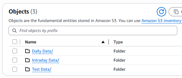
Since we’re working with daily data, the simplest solution is to give each ticker its own folder.

We’ll structure it like this: Daily Data/[TICKER_NAME]

So if we want to save data for AAOI, we’ll file it under:

Daily Data/AAOI/AAOI.parquet

Here’s what that looks like on the AWS S3 platform:

Now, it’s totally understandable if the point of this extra separation isn’t immediately obvious.

The key advantage is that each individual ticker file is compressed down to just a few kilobytes. S3 is already highly optimized for fast data transfers, but when each file is that small, we can access huge amounts of data almost instantly.

To demonstrate the speed advantage, we’ll run a quick sample backtest.

One version will pull daily data for 10 stocks in our investing universe using the S3 Parquet folder structure. The other will pull the same data from the larger, messier imported dataset.

It’s a crude test, but even with the overhead of “talking” to the S3 server and navigating the folder structure, this approach was nearly 3x faster than working from the large dataset stored locally which didn’t require any online querying at all.

Final Thoughts

If you’re going to take this quantitative trading stuff seriously, you’re going to end up running hundreds, maybe thousands, of tests that lead to absolutely nothing. That’s just part of the game.

Eventually, though, you’ll find something.

Ahem — if you’ve been following along and replicated our time-series momentum strategy from a few months ago, then yeah, we’re literally putting a real alpha in your hands that we’re actually making money with — it’s kinda just levered beta, but still. Go get rich. (Kidding… kinda.)

The point is, once you’ve deliberately structured your infrastructure for the “fail fast” approach, everything changes. You can invalidate bad ideas as quickly as you validate the good ones.

Now, if a lot of the terms we covered today were jargon, don’t feel bad: outside of full-time data engineers and quant developers, most people have never touched Parquet files or S3 buckets.

You can of course still get by doing things your own way, but hopefully, this gave you a glimpse into what more structured, scalable infrastructure looks like when applied specifically to quantitative trading.

---

In our first Volatility Trading Bible, we walked through some more infrastructure like this — SQL tables on AWS, automated trading servers; but we’ve gotten a lot better since then. Not just in the quality of our strategies, but also in how we approach infrastructure with current best practices.

We have a vision to essentially package these real-world infrastructure concepts and real-world strategies that actually work and scale into 1 definitive series that you won’t find anywhere else on the planet.

We’re building something serious and if you’ve made it this far, you’re probably the kind of reader we’re doing it for.

Also, definitely join The Quant’s Playbook Discord. Talk shop about the strategies running, ones you’re running on your own, questions, or just stay in the loop.

---

Good luck, and happy trading. 🫡🫡

---

Still need to scratch that itch? You might enjoy these:

• A Junior Quant's Guide to +EV Options Trading

  • Basically, it’s how to tell if your trade idea is already priced in and whether an option is truly underpriced or just a bad bet.

• A Junior Quant's Guide to Chasing Vol and Shorting Stocks

  • The first step in our descent into short selling, kicking off with a hands-on experiment in volatility clustering.

• Quant Galore Crypto #002: Onboarding

  • We’re not done with our crypto experiments. This guide gets you fully set up to follow along with the quant-driven strategies we’ve got cooking.