We Did It. We've Solved The Options Market. [Code Included]

Our last model made some money. Then it made some more money. And now, we're making even more.

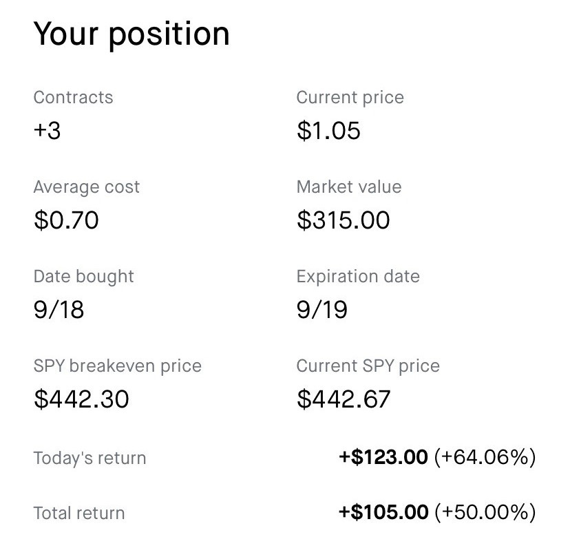
In the last installation of our series on applying machine learning to option markets, we went backwards in time to see if our approach actually had long-term alpha or if we were just getting lucky. After pulling the data as far back as we possibly could, we proved that it wasn’t just chance:

Turbo-Charging The ARIMAX Option System [Code Included]

But here at The Quant’s Playbook, we don’t believe in moderation. If our models accurately predict X% of the time and have historically generated an X% return, why stop there? — In theory, if we just repeat the same research process, building on the research of yesteryear, we’ll wind up with higher accuracies, and more importantly, more money.

So, that’s exactly what we did.

As a token of gratitude for your continued readership, I will include detailed instructions below on how you can deploy and automate the entire pipeline to the cloud so that the model predictions are sent to you daily without you having to lift a finger.

There is a lot of ground to cover, so without further ado, let’s dive right in.

One Market, Two Perspectives

Despite the forthcoming changes, our research objective has remained the same: to predict the direction of overnight S&P 500 returns. Previously, we found success by using data related to the component drivers of the index, but we want to explore whether or not any information can be extracted from just option markets.

But in order for us to extract information from the options market, it will be helpful, if not mandatory, to create our own internal model of this market. To do this, we’ll need a few tools.

The Binomial Pricing Model

Because we want to create our own internal view of markets, we’ll first need information on how options are priced and what volatility the existing market expects. You may already be vaguely familiar with the Black-Scholes model, but it is primarily used for pricing European options, and as such, it won’t do us any good when evaluating real-time American options.

There is no 1 single fixed (i.e., closed-form) method of pricing American options, but one that has demonstrated utility in both academia and Wall Street is the binomial options pricing model. The name may sound intimidating, but we’ll make it simple:

Let’s break this down.

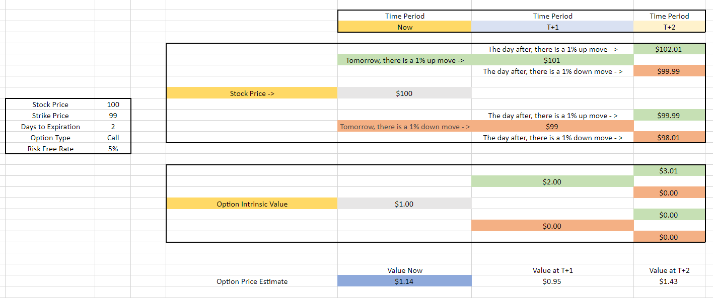
Currently, the stock price is $100 and the risk free rate (treasury rate) is 5%. We want to price a call option that has a strike price of $99 and 2 days to expiration.

As the name bi-nomial suggests, we start with only 2 possibilities: the stock price either goes up, or it goes down. So we create 2 branches (nodes) from the trees that will represent the stock price in 1 day. So, tomorrow, the stock will either be up 1% or down 1%. This is known as a time step.

In one time step (tomorrow), if the stock price is at $101, the option’s intrinsic value (worth at expiration) is $2 since the strike price is $99. If the stock price is at $99, the intrinsic value is $0.00.

Now, let’s go forward another time step. If, in the day after tomorrow, the stock price is up 1% to $102.01, the option’s intrinsic value is worth $3.01. If the stock price is down 1% to $98.01, the intrinsic value is $0.00.

Now that we have the intrinsic values of the option a few steps ahead in time, we want to know what the option should be worth now. To do this, we have to work backwards from the nodes. A formula for this is as follows:

For simplicity, 50% probability of each move is used, but this can be changed by use-case (e.g., expecting lower up probability before fed announcement, etc.)

So, starting 2 time steps ahead, there is a 50% chance the option will be worth $3.01 and a 50% chance it will be worth $0. So, when combined, this gives us a value estimate in 2 days of $1.50. We then discount this by the risk-free rate of 5% to get a price estimate of $1.43.

Price in 2 steps = ((0.5 * 3.01) + (0.5 * 0)) / (1 + .05) = $1.43.

Moving backwards to 1 time step ahead, there is a 50% chance the option will be worth $2.00 and a 50% chance it will be worth $0.00. This gives us a price of $1.00, which when discounted is $0.95.

Price in 1 step = ((0.5*2.00) + (0.5*0)) / (1 + .05) = $0.95

Now moving backwards until today’s time node, there is a 50% chance of the stock price making its move tomorrow, so we now take a weighted average of what the options will be worth, to give us a current price estimate of $1.14.

Price Now = ((0.5 * 0.95) + (0.5*1.43)) / (1 + .05) = $1.14

Finally, this allows us to say, “with a stock price of $100 and an expected stock movement of 1%, a 99 strike call option expiring in 2 days is worth approximately $1.14”.

The actual calculation is a bit more nuanced (no-arbitrage enforcement, more time steps, etc.), but this is the big-picture idea of how it works.

That was kind of intense, so give yourself a quick break.

You may have noticed that we used an assumption of a 1% expected stock move, but how do we actually arrive at an estimate for that? Using historical volatility isn’t effective enough since it doesn’t factor in present or future expectations, so to do this, we have to lean over and copy our classmates’ homework.

The Newton-Raphson Method

While having our own internal model will be important, we still need a way of connecting with the outside world. It could be disastrous if we’re pricing options with an assumed 1% move, but the market is expecting a 5% move. Because of this risk, we need to calibrate with an estimate of what the market expects.

To do this, we need to find the volatility input that makes our model price equal to the price offered by the market. This can be done via brute-force, testing every number from 1 to 1000, but there’s a smarter, faster way.

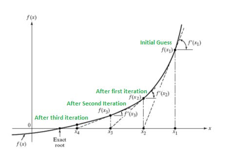
Pulling from the mathematics field of numerical analysis, the Newton-Raphson method is what’s known as a root finding algorithm. Put simply, a root is the input value that makes an equation 0. In our use-case, our equation is (market price - model price). We want to test the values of volatility such that our model price is equal to the market price, a difference (solution) of 0. Let’s walk through an example:

First, we pass in an initial guess of volatility. Remember, volatility is usually calculated on an annualized basis, so if we first guess a 1% expected move, we input ~15.87% (daily vol * sqrt(252 trading days). We then get our model price assuming a 15% implied volatility and see how far away it is from the market’s price of the same option.

Based on how far away the prices are, using a linear approximation, the method tries a different guess, higher or lower. Because it is using an approximation based on sensitivity, it only takes a few iterations to converge at the point where the market’s price is equal to our model’s price.

Once complete, this gives us an internal market-implied volatility for our option. At this point, we now have an internal model of our own prices as well as a real-time estimate of implied volatility.

A New Economic Theory

Before diving into data and modeling, we first need an economic rationale.

This experiment was designed to use features from the options market only, so we won’t use the same S&P factors as before. But luckily, an earlier piece of research provided just the right amount of inspiration:

Hunting Down an ETF Arbitrage