Papa's Got A Brand New Options System [Code Included]

We'll show you what it really means to be an options king.

In recent times, we’ve prioritized our efforts to understanding the style of mainstream strategies that are deployed at major quantitative hedge funds. We discovered that the main forms of profits come from momentum and trend-following based approaches:

Momentum Trading Actually Works... Like, Really, REALLY Well. [Code Included]

Trend Following Is SO Back. [Code Included]

But now, it’s time to come back home.

Historically at The Quant’s Playbook, our focus domain has been short-dated option strategies, whereas our recent focuses have been in the longer end of the delta-1 spectrum. To be frank, although we derive tons of pleasure from the general research angle — we want to make money — lots of it.

So, as we yearn to revert to our roots, we ask ourselves a seemingly simple question:

“If we know what works on the Street and how it works, how hard can it be to put it all together into a short-term working system?”

So, we set out to find an answer — and spoiler alert, we found one.

However, before diving into the meat and bones, we’re shaking up our research process:

Change 1: One Model Doesn’t Fit All

Looking back, when we built a model to capture an effect, say momentum, we would pull data for hundreds of stocks, fit it all into one dataset, divvy it up and then build a model. The thought process was that the larger dataset would give the model plenty of observations so that it could better detect whatever we wanted to capture when it saw new, unseen data.

While this isn’t totally flawed, the approach partially assumes that all stocks exhibit the effect in the same way — which is blatantly untrue. If we want to model how the S&P 500 performs in different regimes, it is unwise to do so with data for shares of Alibaba.

So, looking forward, we will focus more on building models for each asset we want to model something for. A side effect of this is that the model will intrinsically have a smaller dataset size, but it’s a sacrifice we’re willing to make in exchange for logical integrity.

Change 2: Putting The Brakes On Random Forests

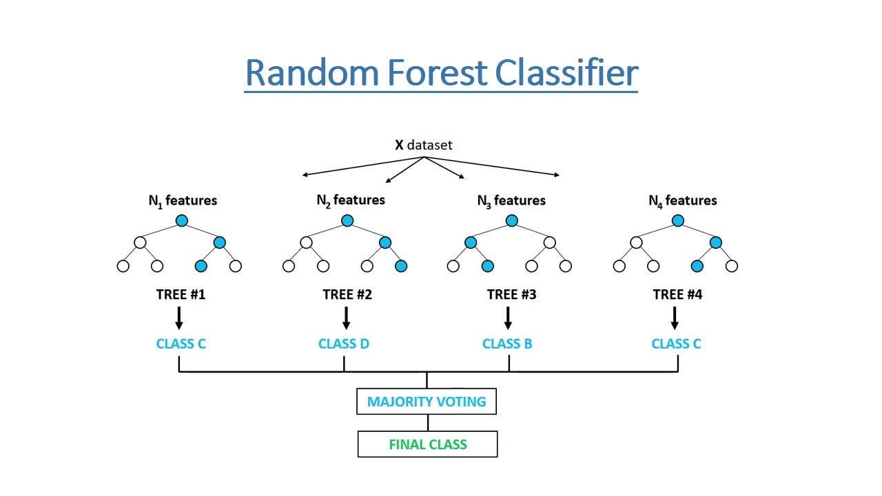
Random forest models have proven their effectiveness to us time and time again, but there’s a slight problem in the way they work.

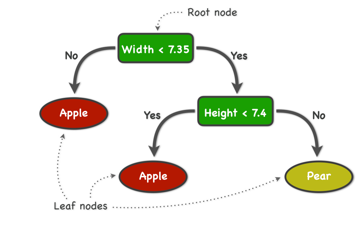
So, in the diagram above (image #2), if we have 7 features, “N(1)” features refers to a tree that uses just 1 feature at the first branch. Looking back to image 1, this can be just using the width of a fruit as the feature used to predict what fruit is given. Doing this random sample of the features ensures variety among the trees, since many are trained using unrelated features.

However, this means that the model output is sort of path-dependent. If we run the model twice and on the second run, the model randomly selects a different starting feature, the outputs can change despite there being no change in the underlying data. In practice, although hundreds of trees are used to mitigate this, probability outputs can vary on a run-to-run basis. The probability changing from 65% to 68% might not be that big of a deal, but a change from 51% to 49% can result in an entirely different prediction!

We are working with serious financial instruments with real-life implications, so we need precision. We need a model who, when it says, “there’s a 75% chance of X event occurring on Jan 1”, will repeat those same words if we run the model again on Jan 15.

In comes our new best friend, gradient boosting.

What first sets gradient boosting apart is how it outputs predictions. Random forests perform the aforementioned sampling, then the output is given as an average or majority-rule of all trees. On the other hand, gradient boosting trains each new tree on the errors of the prior tree. We won’t go into the inner-workings of how it does this, but the big picture idea is that since the trees are run in sequential order, the final output is less influenced by the specific order of the features considered.

This increased model stability isn’t without a tradeoff, naturally. When we train a gradient boosting model to get good at modeling that dataset, we assume that the future will be largely similar to those historical observations — which is generally true, but sometimes it isn’t.

However, that too can be ameliorated:

Change 3: Walk-Forward Testing

In the past, we mainly just split up our dataset by time, trained it on the first section and then passed in the second section as out-of-sample data. This is fine, but in real-life, we wouldn’t be passing in 25 days worth of data at a time — it would be today’s data given to the model trained on everything before today.

So, we need to test our models on a walk-forward basis, for example:

1. We train the model on the first 500 days

2. For each new day, we pass in that days data to get a prediction for

   1. This would return the same prediction we would get if we had taken the model into the real-world

3. We save the prediction and move on to the next day, adding the prior days’ observation to the dataset.

This would allow us to best analyze how the model would’ve performed in the same way we would use it in real-life.

Our goal with these changes are to ensure stability so that when we share the code you see things exactly as we do, and to increase overall robustness as it’s important that our historical testing reflects reality to the fullest extent possible.

Now that we’ve got the technical stuff covered, let’s get into the fun.

A Proprietary Boost

Our goal is simple and ambitious; we want to build a prediction model for what an asset is likely to do tomorrow. We’re able to do that for periods of months and quarters, so why not for a few days?