Insights from a Small-Scale Quantitative Trading Operation

Also, odds optimization, pseudo-arbitrage, and more synthetic data usage.

You may have noticed that it’s been quite awhile since our last post. While we truly regret to keep you waiting, our absence was not without merit.

You see, there’s been some trading — well, kind of a lot of it:

Naturally, from just being out in the field trying things, we learned a lot.

So, today, we’ll be doing a deep dive into what we discovered, some new insights, and a few new strategies that we’re getting ready to launch.

It’s All About The Price, Baby

Although we’re quantitative traders, we briefly lived a past life where we tried to apply the same concepts to sports betting.

To quicky recap, we settled on the conclusion that in sports betting, it’s all about the price. You see, making a net profit from sports betting isn’t about having a good model or understanding the given sport, it’s simply about paying a price that is cheaper than the “fair” price.

Professional bettors essentially just take the fair price from a “sharp” sportsbook like Pinnacle, then search for sportsbooks that provide a deviation from that line. When there’s a sportsbook that’s too far off, you bet big — do that 100 times a day and you’re “guaranteed” a profit.

We expand more on this, along with the results of our own experiment in:

Relative Value Quant Betting: The OddsJam Edition

So, if we can say it all comes down to being a shark — hammering prices when they’re less than fair, can’t that same logic be applied to markets?

To test this idea, we first need a way to convert market prices into implied probabilities. One way of doing this is to use the prices on credit spreads, as explained by the following graphic:

Using the options chain featured above, we can say that at timestamp t, the market implied that there was a 70% probability that the index would be above 5880 at contract expiration — so, 70% represents the “square price” or the fair odds that we should look to improve upon.

Naturally, in similar nature to sports betting odds, this probability will generally end up being accurate. However, also like in sports betting, if odds do anything — they change.

Sometimes, the price of a sports bet at a given sportsbook will change based on things like dollar imbalances (e.g., too much or not enough $ on team A), stale updates, or just general variance. The same applies to markets, where as prices change, so do the odds of a given strike landing out-of-the-money.

To see that in action, take a look at what happened just minutes after the above screenshot was taken:

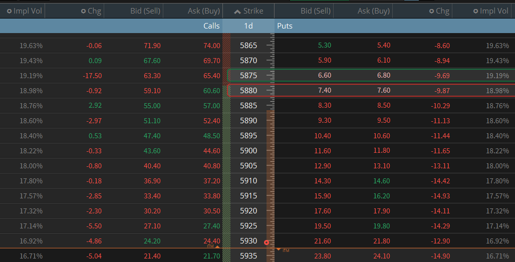
The index rallied upwards by ~30 points, so the same bet that was trading at odds of 70% (1.50 credit) was now trading at odds of 84% (0.80 credit).

So, if we assume that the odds at time t-1, 70%, were the fair odds, our view is that this current price is “rich”/“wrong”.

In +EV betting theory, this would represent a theoretical 14% edge (implied_odds - market_odds). If the odds at 70% are true and we took this bet 1000 times (buying the spread @ 0.80 until it gets back to 1.50), we would theoretically be guaranteed a profit.

Now, of course, knowing which price is the fair one is tricky — just a few minutes after the above screenshot, the odds changed again to 88%.

One simple way is to create a model that just uses the price at time t, say, 9:35 EST, as the true one. Remember, a model is just that — a way of modeling a theory —sometimes it’ll be wrong, but on average it should generally perform okay.

If put into a strategy, we would take all option prices at 9:35 that day and treat it as gospel. So, if at 9:35 the market implied there was an 80% chance for SPX to close above 6000, but a few hours later that probability changed to 25%, we would take that bet.

To quickly test that idea, we can use a modified version of our core SPX strategy:

• Core SPX Strategy: We use the value of the VIX1D index at 9:35 EST, paired with the present market regime to determine the optimal SPX spread to sell that day.

The historical win rate of the strategy is ~80%, so every price at better odds than that (spread price >= 1.05) offers us a theoretical edge. Let’s take a quick look at how the performance differed if instead of trading at the first available price, we only traded with implied odds of 70% (spread price = 1.5).

First, the baseline performance (trading at the first available price after the signal is generated):

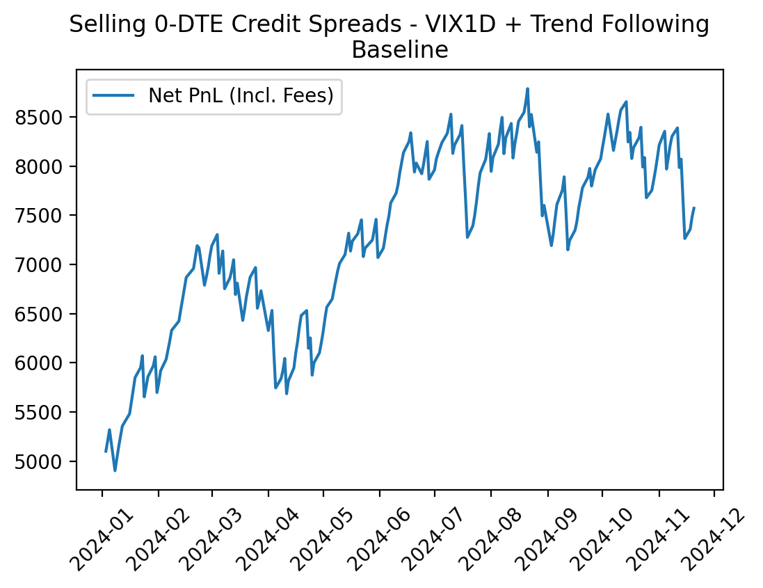
Now, with optimized odds:

As you may have noticed, our base strategy experienced a bit of difficulty recently as the market flattened out and got more volatile (we’ll get to that in a sec), but nevertheless, the version with a 10% odds improvement absolutely dogs the un-optimized version.

Now, of course, there’s no free lunches and getting this optimized price can be a bit tricky.

In a study of a smaller time series, the price of this spread reached $1.5 only ~65% of the time and of that 65%, it ended up actually paying off ~73% of the time. So, when the market implied probability changes, it does end up actually decreasing the probability of the event realizing, but not in a drastic enough way to make the optimization unprofitable.

Nevertheless, if these bets at advantageous prices are peppered into our trades, we can systematically increase and ensure our edge.

Making sure that we actually get filled on those prices though is a fun exercise in algorithmic order execution:

---

Brain Teaser: An Order Execution Puzzle

Scenario: Everyday, the market will offer you $1.00 for something that has an 80% chance of paying off. If it’s wrong, you’ll lose $4.00. You’re smart, so you know that you need a price of at least $1.05 to come out ahead in the long-run. You also know that sometimes, the price gets as high as 1.50, which would cement your edge even further.

Problem: You don’t know what the best price of the day will be, sometimes it’ll be exactly $1.05, sometimes it might even be $4. How do you balance getting filled daily with making sure you’re also exposed to the best prices if/when they arise?

A sample solution is as follows:

1. Your fair probability is 80%, so you start off with a base limit order of $1.05 or the mid price if it’s higher:

   1. np.maximum(1.05, mkt_price)

2. You monitor prices within the first 2 hours and wait for the price of the spread to get to 1.50 (70% prob).

   1. If it doesn’t happen, you collect the full base credit anyway and move onto the next trading day.

   2. If it does, you sell more contracts up to the desired risk limit of the day.

   3. You only wait for 2 hours, since if the prob drastically changes in say, the last 10 minutes of trading, then it’s likely a legitimate bad bet at that point.

As the sample size grows, this process will increase the average trade price and prove to be more efficient than just taking the first available price.

---

Now, while getting an improvement on price is the most surefire way to profits, it won’t totally save a bad strategy.

To see this, let’s take another sample strategy: selling 1-DTE iron condors using the VIX1D value near close.

For this strategy, if we wait until say, 5 minutes before close, that gives us very little room for price improvement. So, rather, we can take the VIX1D value at 2:00 (2 hours before close) and use that as the baseline “true” value. That gives us 2 hours to let prices fluctuate, giving us the best chance to get a fill at an advantageous price.

So, here’s our sample strategy:

1. At 2:00 PM EST, we use the VIX1D to get the implied move for the next day.

2. Based on the implied move, we sell an iron condor directly outside of that range.

   1. We make a profit if the next day’s realized move is less than what the market implied (e.g., market implied prices to move 0.9%, but it only ended up moving 0.5%)

3. Since the prices at 2:00 are our “fair” odds, we use that as the baseline for improvement. So, for the remaining 2 hours we wait for a 10% improvement in price (e.g., “fair” price at 2 = 1.00 | 10% improved price = 1.10).

   1. If the price doesn’t ever reach that amount, the order doesn’t get executed and we don’t take a trade.

      1. We do a 10% improvement in spread price since a 10% difference in implied probability would be too infrequent at strikes this far OTM.

Let’s see how that compared to if we just traded outright every time:

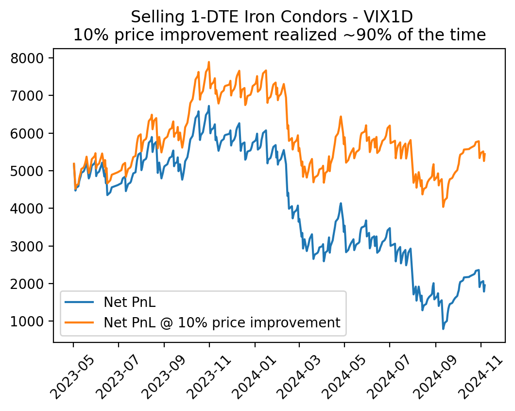
When starting from 2 PM, the price ended up improving by 10% about 90% of the time. However, because pure short vol strategies like this tend to lose in clusters, even getting a 10% improvement doesn’t save the strategy.

So, if you have a strategy that makes money, figuring out the odds (e.g., historical win rate) and delaying execution for price optimization can make you a whole lot more, but the prerequisite is that the strategy is viable in the first place.

Now, with that covered, let’s move onto another matter of business.

Current + New Strategy Updates

At The Quant’s Playbook, we’ve been running 2 quantitative strategies in production.

To quickly recap, we have a strategy that uses a short-term prediction model to predict the next day direction of TSLA’s stock. Based on that prediction, we buy a call or put at near market close and sell it at market open the next day.

Because TSLA routinely experiences volatile moves that outpace implied volatility, its options provide greatly asymmetric returns which allow us to have a positive expected value even if we just go 50/50.

Put simply, this strategy, has been making us rich — month after month:

---

If you’re already a paid subscriber, truly — thank you. ❤️ Your support powers better data, better tools, and better research.

If you’ve been enjoying the work and want to support what we’re building, consider becoming a paid subscriber. It means more than you think and helps us keep doing it right. 🫡

---