A Junior Quant's Guide to Factor Investing

Sometimes, being a quant is about more than just math...

Being a quant is fun, no doubt about it. However, in order for us to be good quants, it’s important that we sometimes take a step back to make sure our financial theory knowledge is in check.

If you’ve ever seen the words “systematic” and “equities” mentioned in tandem, there’s a 90% chance the word “factor” wasn’t too far away. If you’re unfamiliar with factors as a concept, we don’t blame you — quantitative factor investing is one of the most arcane forms of alphas out there. Arcane, but not unprofitable:

So, today we’ll be taking a deep dive into what factors are, why they’re important, and ultimately to understand how it’s relevant and applied in today’s markets.

What Even Is a “Factor”?

Before you can fully understand factors and why they’re useful, we first need to start with the Capital Asset Pricing Model (CAPM). Don’t worry, it’s less daunting than it sounds.

The CAPM model is simply the way to get the expected return of an asset (e.g., stock). Basically, after plugging in some parameters, the model will spit out the return you should expect from holding that particular stock. These inputs include:

• Risk-free rate (Rf): The return you’d get from a no-risk treasury bond.

• Market Return (Rm): The return you’d expect from the broad market. For instance, the average S&P 500 return.

• Beta (B): How sensitive the asset is compared to the the broad market.

• Equity Risk Premium (Rm - Rf): The premium the market offers you for taking on the risk of not just going with a risk-free option.

  • If a risk-free treasury bond pays 5%, but the market will give you on average, 7%, you are essentially being compensated an extra 2% for introducing the risk of the market (7%-5%).

Once you have all of those inputs, you squeeze them all together to get the expected return of a stock. To see why this is useful, let’s calculate the expected returns of a volatile stock (Tesla) and a less volatile one (Walmart):

Expected Return = Risk-free rate + (Beta * Risk Premium)

Expected Return (TSLA) = 5% + (2.44 * 2%) = 9.88%

Expected Return (WMT) = 5% + (0.49 * 2%) = 5.98%

So, the CAPM is essentially a way of saying “In the long-run, on average, we expect this asset to return x%”. If we combined our 2 example stocks into an equal-weighted portfolio (TSLA/WMT), our expected return would be ~7.98% with a beta of ~1.47. We would repeat that for a bunch of other portfolios to generate a curve like this:

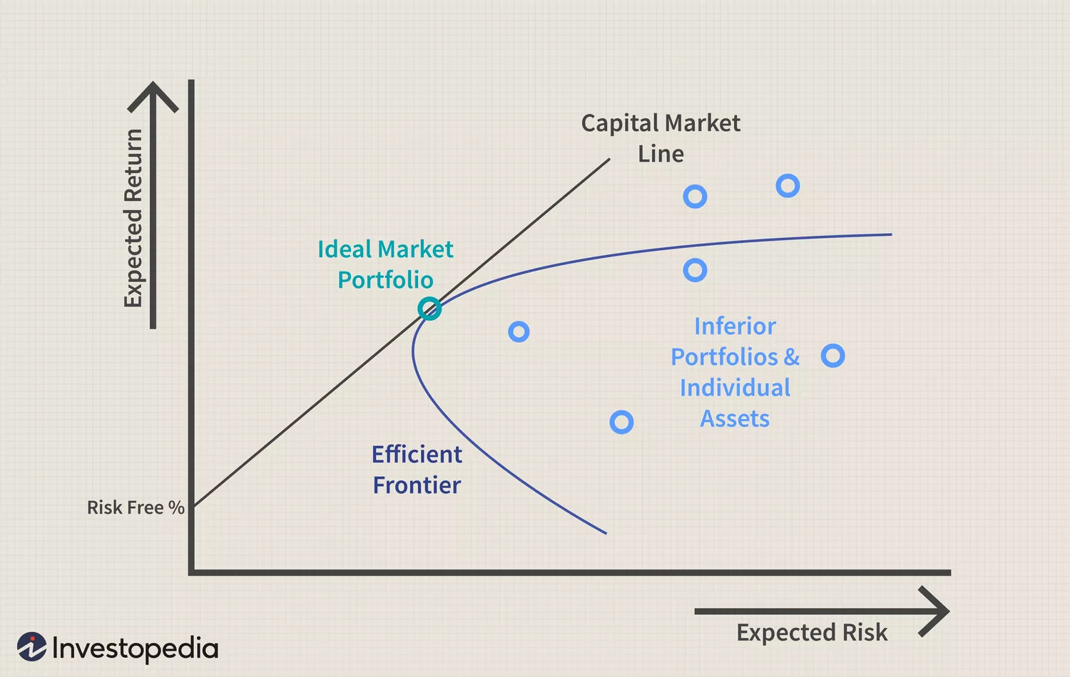
This curve, known as the efficiency frontier, allows us to choose the optimal portfolio where we would be able to have the highest expected return for the lowest amount of risk — the efficient frontier.

Back in the 1960s, this was a Nobel-worthy game changer, but a few decades later, there was a problem. As time went on, these theoretically optimal portfolios began to perform poorly. The CAPM approach is extremely dependent on the beta of the stock, so even if a stock is complete garbage, CAPM will give a high expected return if it’s volatile enough.

So, 30 years later, two guys suggested that the expected return of a stock was dependent on a few more factors:

In 1992, Eugene Fama and Kenneth French introduced The Fama-French 3-Factor Model which modified the CAPM model to account for factors relevant to the specific stock.

Mathematically speaking, the new approach went from:

Expected Return = Risk-free rate + (Beta * Risk Premium)

to

Expected Return = Risk-free rate + (Beta * Risk Premium) + (Beta_of_Factor_1 * Factor_1) + (Beta_of_Factor_2 * Factor_2)

• The beta of a factor essentially represents how the price performance changes with changes in the factor. So, if the share price becomes higher with more volatility when the value factor becomes higher, the beta of the value factor increases.

In the 30 years since that publication, the consensus of what works has narrowed on a few major factors:

• Size: Over a long horizon, stocks with smaller market capitalizations tend to outperform those with larger market caps.

• Value: Value stocks tend to outperform expensive stocks.

• Momentum: Stocks that have demonstrated strong momentum historically will continue to demonstrate it in the future.

• Volatility: Stocks with lower volatility tend to outperform those with higher volatility.

Some of those factors might seem a bit vague, so let’s see a few examples of how it’s done in the real world:

How Do You Actually USE Factors?

To begin, we’ll start with the value factor.